Machine Learning: the Titanic dataset¶

If you want to try out this notebook with a live Python kernel, use mybinder:

In the following is a more involved machine learning example, in which we will use a larger variety of methods in veax to do data cleaning, feature engineering, pre-processing and finally to train a couple of models. To do this, we will use the well known Titanic dataset. Our task is to predict which passengers are more likely to have survived the disaster.

Before we begin, there are two important notes to consider: - The following example is not to provide a competitive score for any competitions that might use the Titanic dataset. It’s primary goal is to show how various methods provided by vaex and vaex.ml can be used to clean data, create new features, and do general data manipulations in a machine learning context. - While the Titanic dataset is rather small in side, all the methods and operations presented in the solution below will work on a dataset of arbitrary size, as long as the data fits on the hard-drive of your machine.

Now, with that out of the way, let’s get started!

[1]:

import vaex
import vaex.ml

import numpy as np
import matplotlib.pyplot as plt

Adjusting `matplotlib` parmeters¶

Intermezzo: we modify some of the matplotlib default settings, just to make the plots a bit more legible.

[2]:

SMALL_SIZE = 12
MEDIUM_SIZE = 14
BIGGER_SIZE = 16

plt.rc('font', size=SMALL_SIZE)          # controls default text sizes
plt.rc('axes', titlesize=SMALL_SIZE)     # fontsize of the axes title
plt.rc('axes', labelsize=MEDIUM_SIZE)    # fontsize of the x and y labels
plt.rc('xtick', labelsize=SMALL_SIZE)    # fontsize of the tick labels
plt.rc('ytick', labelsize=SMALL_SIZE)    # fontsize of the tick labels
plt.rc('legend', fontsize=SMALL_SIZE)    # legend fontsize
plt.rc('figure', titlesize=BIGGER_SIZE)  # fontsize of the figure title

Get the data¶

First of all we need to read in the data. Since the Titanic dataset is quite well known for trying out different classification algorithms, as well as commonly used as a teaching tool for aspiring data scientists, it ships (no pun intended) together with vaex.ml. So let’s read it in, see the description of its contents, and get a preview of the data.

[3]:

# Load the titanic dataset
df = vaex.datasets.titanic()

# See the description
df.info()

titanic

rows: 1,309

Columns:

column	type	unit	description	expression
pclass	int64
survived	bool
name	str
sex	str
age	float64
sibsp	int64
parch	int64
ticket	str
fare	float64
cabin	str
embarked	str
boat	str
body	float64
home_dest	str

Data:

#	pclass	survived	name	sex	age	sibsp	parch	ticket	fare	cabin	embarked	boat	body	home_dest
0	1	True	Allen, Miss. Elisabeth Walton	female	29.0	0	0	24160	211.3375	B5	S	2	nan	St Louis, MO
1	1	True	Allison, Master. Hudson Trevor	male	0.9167	1	2	113781	151.55	C22 C26	S	11	nan	Montreal, PQ / Chesterville, ON
2	1	False	Allison, Miss. Helen Loraine	female	2.0	1	2	113781	151.55	C22 C26	S	--	nan	Montreal, PQ / Chesterville, ON
3	1	False	Allison, Mr. Hudson Joshua Creighton	male	30.0	1	2	113781	151.55	C22 C26	S	--	135.0	Montreal, PQ / Chesterville, ON
4	1	False	Allison, Mrs. Hudson J C (Bessie Waldo Daniels)	female	25.0	1	2	113781	151.55	C22 C26	S	--	nan	Montreal, PQ / Chesterville, ON
...	...	...	...	...	...	...	...	...	...	...	...	...	...	...
1,304	3	False	Zabour, Miss. Hileni	female	14.5	1	0	2665	14.4542	--	C	--	328.0	--
1,305	3	False	Zabour, Miss. Thamine	female	nan	1	0	2665	14.4542	--	C	--	nan	--
1,306	3	False	Zakarian, Mr. Mapriededer	male	26.5	0	0	2656	7.225	--	C	--	304.0	--
1,307	3	False	Zakarian, Mr. Ortin	male	27.0	0	0	2670	7.225	--	C	--	nan	--
1,308	3	False	Zimmerman, Mr. Leo	male	29.0	0	0	315082	7.875	--	S	--	nan	--

Shuffling¶

From the preview of the DataFrame we notice that the data is sorted alphabetically by name and by passenger class. Thus we need to shuffle it before we split it into train and test sets.

[4]:

# The dataset is ordered, so let's shuffle it
df = df.shuffle(random_state=31)

Shuffling for large datasets¶

As mentioned in The Iris tutorial, you are likely to get a better performance if you export to disk your shuffled dataset, especially when the dataset is larger in size:

df.shuffle().export("shuffled.hdf5")
df = vaex.open("shuffled.hdf5")
df_train, df_test = df.ml.train_test_split(test_size=0.2)

Split into train and test¶

Once the data is shuffled, let’s split it into train and test sets. The test set will comprise 20% of the data. Note that we do not shuffle the data for you, since vaex cannot assume your data fits into memory, you are responsible for either writing it in shuffled order on disk, or shuffle it in memory (the previous step).

[5]:

# Train and test split, no shuffling occurs
df_train, df_test = df.ml.train_test_split(test_size=0.2, verbose=False)

Sanity checks¶

Before we move on to process the data, let’s verify that our train and test sets are “similar” enough. We will not be very rigorous here, but just look at basic statistics of some of the key features.

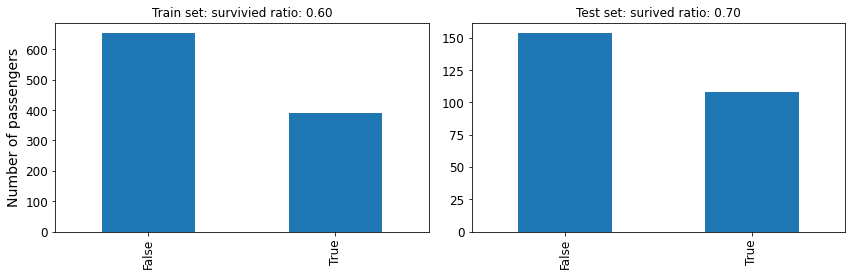
For starters, let’s check that the fraction of survivals is similar between the train and test sets.

[6]:

# Inspect the target variable
train_survived_value_counts = df_train.survived.value_counts()
test_survived_value_counts = df_test.survived.value_counts()


plt.figure(figsize=(12, 4))

plt.subplot(121)
train_survived_value_counts.plot.bar()
train_sex_ratio = train_survived_value_counts[True]/train_survived_value_counts[False]
plt.title(f'Train set: survivied ratio: {train_sex_ratio:.2f}')
plt.ylabel('Number of passengers')

plt.subplot(122)
test_survived_value_counts.plot.bar()
test_sex_ratio = test_survived_value_counts[True]/test_survived_value_counts[False]
plt.title(f'Test set: surived ratio: {test_sex_ratio:.2f}')


plt.tight_layout()
plt.show()

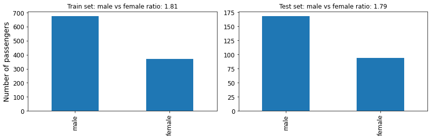
Next up, let’s check whether the ratio of male to female passengers is not too dissimilar between the two sets.

[7]:

# Check the sex balance
train_sex_value_counts = df_train.sex.value_counts()
test_sex_value_counts = df_test.sex.value_counts()

plt.figure(figsize=(12, 4))

plt.subplot(121)
train_sex_value_counts.plot.bar()
train_sex_ratio = train_sex_value_counts['male']/train_sex_value_counts['female']
plt.title(f'Train set: male vs female ratio: {train_sex_ratio:.2f}')
plt.ylabel('Number of passengers')

plt.subplot(122)
test_sex_value_counts.plot.bar()
test_sex_ratio = test_sex_value_counts['male']/test_sex_value_counts['female']
plt.title(f'Test set: male vs female ratio: {test_sex_ratio:.2f}')


plt.tight_layout()
plt.show()

Finally, lets check that the relative number of passenger per class is similar between the train and test sets.

[8]:

# Check the class balance
train_pclass_value_counts = df_train.pclass.value_counts() / len(df_train)
test_pclass_value_counts = df_test.pclass.value_counts() / len(df_test)

plt.figure(figsize=(12, 4))

plt.subplot(121)
plt.title('Train set: passenger class')
plt.ylabel('Fraction of passengers')
train_pclass_value_counts.plot.bar()

plt.subplot(122)
plt.title('Test set: passenger class')
test_pclass_value_counts.plot.bar()

plt.tight_layout()
plt.show()

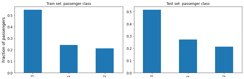
From the above diagnostics, we are satisfied that, at least in these few categories, the train and test are similar enough, and we can move forward.

Feature engineering¶

In this section we will use vaex to create meaningful features that will be used to train a classification model. To start with, let’s get a high level overview of the training data.

[9]:

df_train.describe()

[9]:

	pclass	survived	name	sex	age	sibsp	parch	ticket	fare	cabin	embarked	boat	body	home_dest
data_type	int64	bool	string	string	float64	int64	int64	string	float64	string	string	string	float64	string
count	1047	1047	1047	1047	841	1047	1047	1047	1046	233	1046	380	102	592
NA	0	0	0	0	206	0	0	0	1	814	1	667	945	455
mean	2.3075453677172875	0.3744030563514804	--	--	29.565299286563608	0.5100286532951289	0.3982808022922636	--	32.92609101338429	--	--	--	159.6764705882353	--
std	0.833269	0.483968	--	--	14.161953	1.071309	0.890852	--	50.678261	--	--	--	96.220759	--
min	1	False	--	--	0.1667	0	0	--	0.0	--	--	--	1.0	--
max	3	True	--	--	80.0	8	9	--	512.3292	--	--	--	327.0	--

Imputing¶

We notice that there are 3 columns that have missing data, so our first task will be to impute the missing values with suitable substitutes. This is our strategy:

age: impute with the median age value
fare: impute with the mean fare of the 5 most common values.
cabin: impute with “M” for “Missing”
Embarked: Impute with with the most common value.

[10]:

# Handle missing values

# Age - just do the median of the training set for now
fill_age = df_train.percentile_approx(expression='age', percentage=50.0)
# For some numpy versions the `np.percentile` method is broken and returns nan.
# As a failsafe, in those cases fill with the mean.
if np.isnan(fill_age):
    fill_age = df_train.mean(expression='age')
df_train['age'] = df_train.age.fillna(value=fill_age)

# Fare: the mean of the 5 most common ticket prices.
fill_fares = df_train.fare.value_counts(dropna=True)
fill_fare = fill_fares.iloc[:5].index.values.mean()
df_train['fare'] = df_train.fare.fillna(value=fill_fare)

# Cabing: this is a string column so let's mark it as "M" for "Missing"
df_train['cabin'] = df_train.cabin.fillna(value='M')

# Embarked: Similar as for Cabin, let's mark the missing values with "U" for unknown
fill_embarked = df_train.embarked.value_counts(dropna=True).index[0]
df_train['embarked'] = df_train.embarked.fillna(value=fill_embarked)

String processing¶

Next up, let’s engineer some new, more meaningful features out of the “raw” data that is present in the dataset. Starting with the name of the passengers, we are going to extract the titles, as well as we are going to count the number of words a name contains. These features can be a loose proxy to the age and status of the passengers.

[11]:

# Engineer features from the names

# Titles
df_train['name_title'] = df_train['name'].str.replace('.* ([A-Z][a-z]+)\..*', "\\1", regex=True)
display(df_train['name_title'])

# Number of words in the name
df_train['name_num_words'] = df_train['name'].str.count("[ ]+", regex=True) + 1
display(df_train['name_num_words'])

Expression = name_title
Length: 1,047 dtype: large_string (column)
------------------------------------------
   0      Mr
   1      Mr
   2     Mrs
   3    Miss
   4      Mr
    ...
1042  Master
1043     Mrs
1044  Master
1045      Mr
1046      Mr

Expression = name_num_words
Length: 1,047 dtype: int64 (column)
-----------------------------------
   0  3
   1  4
   2  5
   3  4
   4  4
  ...
1042  4
1043  6
1044  4
1045  4
1046  3

From the cabin colum, we will engineer 3 features: - “deck”: extacting the deck on which the cabin is located, which is encoded in each cabin value; - “multi_cabin: a boolean feature indicating whether a passenger is allocated more than one cabin - “has_cabin”: since there were plenty of values in the original cabin column that had missing values, we are just going to build a feature which tells us whether a passenger had an assigned cabin or not.

[12]:

#  Extract the deck
df_train['deck'] = df_train.cabin.str.slice(start=0, stop=1)
display(df_train['deck'])

# Passengers under which name have several rooms booked, these are all for 1st class passengers
df_train['multi_cabin'] = ((df_train.cabin.str.count(pat='[A-Z]', regex=True) > 1) &\
                           ~(df_train.deck == 'F')).astype('int')
display(df_train['multi_cabin'])

# Out of these, cabin has the most missing values, so let's create a feature tracking if a passenger had a cabin
df_train['has_cabin'] = df_train.cabin.notna().astype('int')
display(df_train['has_cabin'])

Expression = deck
Length: 1,047 dtype: string (column)
------------------------------------
   0  M
   1  B
   2  M
   3  M
   4  M
  ...
1042  M
1043  M
1044  M
1045  B
1046  M

Expression = multi_cabin
Length: 1,047 dtype: int64 (column)
-----------------------------------
   0  0
   1  0
   2  0
   3  0
   4  0
  ...
1042  0
1043  0
1044  0
1045  1
1046  0

Expression = has_cabin
Length: 1,047 dtype: int64 (column)
-----------------------------------
   0  1
   1  1
   2  1
   3  1
   4  1
  ...
1042  1
1043  1
1044  1
1045  1
1046  1

More features¶

There are two features that give an indication whether a passenger is travelling alone, or with a famly. These are the “sibsp” and “parch” columns that tell us the number of siblinds or spouses and the number of parents or children each passenger has on-board respectively. We are going to use this information to build two columns: - “family_size” the size of the family of each passenger; - “is_alone” an additional boolean feature which indicates whether a passenger is traveling without their family.

[13]:

# Size of family that are on board: passenger + number of siblings, spouses, parents, children.
df_train['family_size'] = (df_train.sibsp + df_train.parch + 1)
display(df_train['family_size'])

# Whether or not a passenger is alone
df_train['is_alone'] = (df_train.family_size == 0).astype('int')
display(df_train['is_alone'])

Expression = family_size
Length: 1,047 dtype: int64 (column)
-----------------------------------
   0  1
   1  1
   2  3
   3  4
   4  1
  ...
1042  8
1043  2
1044  3
1045  2
1046  1

Expression = is_alone
Length: 1,047 dtype: int64 (column)
-----------------------------------
   0  0
   1  0
   2  0
   3  0
   4  0
  ...
1042  0
1043  0
1044  0
1045  0
1046  0

Finally, let’s create two new features: - age \(\times\) class - fare per family member, i.e. fare \(/\) family_size

[14]:

# Create new features
df_train['age_times_class'] = df_train.age * df_train.pclass

# fare per person in the family
df_train['fare_per_family_member'] = df_train.fare / df_train.family_size

Modeling (part 1): gradient boosted trees¶

Since this dataset contains a lot of categorical features, we will start with a tree based model. This we will gear the following feature pre-processing towards the use of tree-based models.

Feature pre-processing for boosted tree models¶

The features “sex”, “embarked”, and “deck” can be simply label encoded. The feature “name_tite” contains certain a larger degree of cardinality, relative to the size of the training set, and in this case we will use the Frequency Encoder.

[15]:

label_encoder = vaex.ml.LabelEncoder(features=['sex', 'embarked', 'deck'], allow_unseen=True)
df_train = label_encoder.fit_transform(df_train)

# While doing a transform, previously unseen values will be encoded as "zero".
frequency_encoder = vaex.ml.FrequencyEncoder(features=['name_title'], unseen='zero')
df_train = frequency_encoder.fit_transform(df_train)
df_train

[15]:

#	pclass	survived	name	sex	age	sibsp	parch	ticket	fare	cabin	embarked	boat	body	home_dest	name_title	name_num_words	deck	multi_cabin	has_cabin	family_size	is_alone	age_times_class	fare_per_family_member	label_encoded_sex	label_encoded_embarked	label_encoded_deck	frequency_encoded_name_title
0	3	False	Stoytcheff, Mr. Ilia	male	19.0	0	0	349205	7.8958	M	S	--	nan	--	Mr	3	M	0	1	1	0	57.0	7.8958	1	1	0	0.5787965616045845
1	1	False	Payne, Mr. Vivian Ponsonby	male	23.0	0	0	12749	93.5	B24	S	--	nan	Montreal, PQ	Mr	4	B	0	1	1	0	23.0	93.5	1	1	1	0.5787965616045845
2	3	True	Abbott, Mrs. Stanton (Rosa Hunt)	female	35.0	1	1	C.A. 2673	20.25	M	S	A	nan	East Providence, RI	Mrs	5	M	0	1	3	0	105.0	6.75	0	1	0	0.1451766953199618
3	2	True	Hocking, Miss. Ellen "Nellie"	female	20.0	2	1	29105	23.0	M	S	4	nan	Cornwall / Akron, OH	Miss	4	M	0	1	4	0	40.0	5.75	0	1	0	0.20152817574021012
4	3	False	Nilsson, Mr. August Ferdinand	male	21.0	0	0	350410	7.8542	M	S	--	nan	--	Mr	4	M	0	1	1	0	63.0	7.8542	1	1	0	0.5787965616045845
...	...	...	...	...	...	...	...	...	...	...	...	...	...	...	...	...	...	...	...	...	...	...	...	...	...	...	...
1,042	3	False	Goodwin, Master. Sidney Leonard	male	1.0	5	2	CA 2144	46.9	M	S	--	nan	Wiltshire, England Niagara Falls, NY	Master	4	M	0	1	8	0	3.0	5.8625	1	1	0	0.045845272206303724
1,043	3	False	Ahlin, Mrs. Johan (Johanna Persdotter Larsson)	female	40.0	1	0	7546	9.475	M	S	--	nan	Sweden Akeley, MN	Mrs	6	M	0	1	2	0	120.0	4.7375	0	1	0	0.1451766953199618
1,044	3	True	Johnson, Master. Harold Theodor	male	4.0	1	1	347742	11.1333	M	S	15	nan	--	Master	4	M	0	1	3	0	12.0	3.7111	1	1	0	0.045845272206303724
1,045	1	False	Baxter, Mr. Quigg Edmond	male	24.0	0	1	PC 17558	247.5208	B58 B60	C	--	nan	Montreal, PQ	Mr	4	B	1	1	2	0	24.0	123.7604	1	0	1	0.5787965616045845
1,046	3	False	Coleff, Mr. Satio	male	24.0	0	0	349209	7.4958	M	S	--	nan	--	Mr	3	M	0	1	1	0	72.0	7.4958	1	1	0	0.5787965616045845

Once all the categorical data is encoded, we can select the features we are going to use for training the model.

[16]:

# features to use for the trainin of the boosting model
encoded_features = df_train.get_column_names(regex='^freque|^label')
features = encoded_features + ['multi_cabin', 'name_num_words',
                               'has_cabin', 'is_alone',
                               'family_size', 'age_times_class',
                               'fare_per_family_member',
                               'age', 'fare']

# Preview the feature matrix
df_train[features].head(5)

[16]:

#	label_encoded_sex	label_encoded_embarked	label_encoded_deck	frequency_encoded_name_title	name_num_words	has_cabin	family_size	age_times_class	fare_per_family_member	age	fare
0	1	1	0	0.578797	3	1	1	57	7.8958	19	7.8958
1	1	1	1	0.578797	4	1	1	23	93.5	23	93.5
2	0	1	0	0.145177	5	1	3	105	6.75	35	20.25
3	0	1	0	0.201528	4	1	4	40	5.75	20	23
4	1	1	0	0.578797	4	1	1	63	7.8542	21	7.8542

Estimator: xgboost ¶

Now let’s feed this data into an a tree based estimator. In this example we will use xgboost. In principle, any algorithm that follows the scikit-learn API convention, i.e. it contains the .fit, .predict methods is compatable with vaex. However, the data will be materialized, i.e. will be read into memory before it is passed on to the estimators. We are hard at work trying to make at least some of the estimators from scikit-learn run out-of-core!

[17]:

import xgboost
import vaex.ml.sklearn

# Instantiate the xgboost model normally, using the scikit-learn API
xgb_model = xgboost.sklearn.XGBClassifier(max_depth=11,
                                          learning_rate=0.1,
                                          n_estimators=500,
                                          subsample=0.75,
                                          colsample_bylevel=1,
                                          colsample_bytree=1,
                                          scale_pos_weight=1.5,
                                          reg_lambda=1.5,
                                          reg_alpha=5,
                                          n_jobs=8,
                                          random_state=42,
                                          use_label_encoder=False,
                                          verbosity=0)

# Make it work with vaex (for the automagic pipeline and lazy predictions)
vaex_xgb_model = vaex.ml.sklearn.Predictor(features=features,
                                           target='survived',
                                           model=xgb_model,
                                           prediction_name='prediction_xgb')
# Train the model
vaex_xgb_model.fit(df_train)
# Get the prediction of the model on the training data
df_train = vaex_xgb_model.transform(df_train)

# Preview the resulting train dataframe that contans the predictions
df_train

[17]:

#	pclass	survived	name	sex	age	sibsp	parch	ticket	fare	cabin	embarked	boat	body	home_dest	name_title	name_num_words	deck	multi_cabin	has_cabin	family_size	is_alone	age_times_class	fare_per_family_member	label_encoded_sex	label_encoded_embarked	label_encoded_deck	frequency_encoded_name_title	prediction_xgb
0	3	False	Stoytcheff, Mr. Ilia	male	19.0	0	0	349205	7.8958	M	S	--	nan	--	Mr	3	M	0	1	1	0	57.0	7.8958	1	1	0	0.5787965616045845	0
1	1	False	Payne, Mr. Vivian Ponsonby	male	23.0	0	0	12749	93.5	B24	S	--	nan	Montreal, PQ	Mr	4	B	0	1	1	0	23.0	93.5	1	1	1	0.5787965616045845	0
2	3	True	Abbott, Mrs. Stanton (Rosa Hunt)	female	35.0	1	1	C.A. 2673	20.25	M	S	A	nan	East Providence, RI	Mrs	5	M	0	1	3	0	105.0	6.75	0	1	0	0.1451766953199618	1
3	2	True	Hocking, Miss. Ellen "Nellie"	female	20.0	2	1	29105	23.0	M	S	4	nan	Cornwall / Akron, OH	Miss	4	M	0	1	4	0	40.0	5.75	0	1	0	0.20152817574021012	1
4	3	False	Nilsson, Mr. August Ferdinand	male	21.0	0	0	350410	7.8542	M	S	--	nan	--	Mr	4	M	0	1	1	0	63.0	7.8542	1	1	0	0.5787965616045845	0
...	...	...	...	...	...	...	...	...	...	...	...	...	...	...	...	...	...	...	...	...	...	...	...	...	...	...	...	...
1,042	3	False	Goodwin, Master. Sidney Leonard	male	1.0	5	2	CA 2144	46.9	M	S	--	nan	Wiltshire, England Niagara Falls, NY	Master	4	M	0	1	8	0	3.0	5.8625	1	1	0	0.045845272206303724	0
1,043	3	False	Ahlin, Mrs. Johan (Johanna Persdotter Larsson)	female	40.0	1	0	7546	9.475	M	S	--	nan	Sweden Akeley, MN	Mrs	6	M	0	1	2	0	120.0	4.7375	0	1	0	0.1451766953199618	0
1,044	3	True	Johnson, Master. Harold Theodor	male	4.0	1	1	347742	11.1333	M	S	15	nan	--	Master	4	M	0	1	3	0	12.0	3.7111	1	1	0	0.045845272206303724	1
1,045	1	False	Baxter, Mr. Quigg Edmond	male	24.0	0	1	PC 17558	247.5208	B58 B60	C	--	nan	Montreal, PQ	Mr	4	B	1	1	2	0	24.0	123.7604	1	0	1	0.5787965616045845	0
1,046	3	False	Coleff, Mr. Satio	male	24.0	0	0	349209	7.4958	M	S	--	nan	--	Mr	3	M	0	1	1	0	72.0	7.4958	1	1	0	0.5787965616045845	0

Notice that in the above cell block, we call .transform on the vaex_xgb_model object. This adds the “prediction_xgb” column as virtual column in the output dataframe. This can be quite convenient when calculating various metrics and making diagnosic plots. Of course, one can call a .predict on the vaex_xgb_model object, which returns an in-memory numpy array object housing the predictions.

Performance on training set¶

Anyway, let’s see what the performance is of the model on the training set. First let’s create a convenience function that will help us get multiple metrics at once.

[18]:

from sklearn.metrics import accuracy_score, f1_score, roc_auc_score
def binary_metrics(y_true, y_pred):
    acc = accuracy_score(y_true=y_true, y_pred=y_pred)
    f1 = f1_score(y_true=y_true, y_pred=y_pred)
    roc = roc_auc_score(y_true=y_true, y_score=y_pred)
    print(f'Accuracy: {acc:.3f}')
    print(f'f1 score: {f1:.3f}')
    print(f'roc-auc: {roc:.3f}')

Now let’s check the performance of the model on the training set.

[19]:

print('Metrics for the training set:')
binary_metrics(y_true=df_train.survived.values, y_pred=df_train.prediction_xgb.values)

Metrics for the training set:
Accuracy: 0.924
f1 score: 0.896
roc-auc: 0.914

Automatic pipelines¶

Now, let’s inspect the performance of the model on the test set. You probably noticed that, unlike when using other libraries, we did not bother to create a pipeline while doing all the cleaning, inputing, feature engineering and categorial encoding. Well, we did not explicitly create a pipeline. In fact veax keeps track of all the changes one applies to a DataFrame in something called a state. A state is the place which contains all the informations regarding, for instance, the virtual columns we’ve created, which includes the newly engineered features, the categorically encoded columns, and even the model prediction! So all we need to do, is to extract the state from the training DataFrame, and apply it to the test DataFrame.

[20]:

# state transfer to the test set
state = df_train.state_get()
df_test.state_set(state)

# Preview of the "transformed" test set
df_test.head(5)

[20]:

#	pclass	survived	name	sex	age	parch	ticket	fare	cabin	embarked	boat	body	home_dest	name_title	name_num_words	deck	has_cabin	family_size	age_times_class	fare_per_family_member	label_encoded_sex	label_encoded_embarked	label_encoded_deck	frequency_encoded_name_title	prediction_xgb
0	3	False	O'Connor, Mr. Patrick	male	28.032	0	366713	7.75	M	Q	--	nan	--	Mr	3	M	1	1	84.096	7.75	1	2	0	0.578797	0
1	3	False	Canavan, Mr. Patrick	male	21	0	364858	7.75	M	Q	--	nan	Ireland Philadelphia, PA	Mr	3	M	1	1	63	7.75	1	2	0	0.578797	0
2	1	False	Ovies y Rodriguez, Mr. Servando	male	28.5	0	PC 17562	27.7208	D43	C	--	189	?Havana, Cuba	Mr	5	D	1	1	28.5	27.7208	1	0	4	0.578797	1
3	3	False	Windelov, Mr. Einar	male	21	0	SOTON/OQ 3101317	7.25	M	S	--	nan	--	Mr	3	M	1	1	63	7.25	1	1	0	0.578797	0
4	2	True	Shelley, Mrs. William (Imanita Parrish Hall)	female	25	1	230433	26	M	S	12	nan	Deer Lodge, MT	Mrs	6	M	1	2	50	13	0	1	0	0.145177	1

Notice that once we apply the state from the train to the test set, the test DataFrame contains all the features we created or modified in the training data, and even the predictions of the xgboost model!

The state is a simple Python dictionary, which can be easily stored as JSON to disk, which makes it very easy to deploy.

Performance on test set¶

Now it is trivial to check the model performance on the test set:

[21]:

print('Metrics for the test set:')
binary_metrics(y_true=df_test.survived.values, y_pred=df_test.prediction_xgb.values)

Metrics for the test set:
Accuracy: 0.786
f1 score: 0.728
roc-auc: 0.773

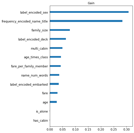
Feature importance¶

Let’s now look at the feature importance of the xgboost model.

[22]:

plt.figure(figsize=(6, 9))

ind = np.argsort(xgb_model.feature_importances_)[::-1]
features_sorted = np.array(features)[ind]
importances_sorted = xgb_model.feature_importances_[ind]

plt.barh(y=range(len(features)), width=importances_sorted, height=0.2)
plt.title('Gain')
plt.yticks(ticks=range(len(features)), labels=features_sorted)
plt.gca().invert_yaxis()
plt.show()

Modeling (part 2): Linear models & Ensembles¶

Given the randomness of the Titanic dataset , we can be satisfied with the performance of xgboost model above. Still, it is always usefull to try a variety of models and approaches, especially since vaex makes makes this process rather simple.

In the following part we will use a couple of linear models as our predictors, this time straight from scikit-learn. This requires us to pre-process the data in a slightly different way.

Feature pre-processing for linear models¶

When using linear models, the safest option is to encode categorical variables with the one-hot encoding scheme, especially if they have low cardinality. We will do this for the “family_size” and “deck” features. Note that the “sex” feature is already encoded since it has only unique values options.

The “name_title” feature is a bit more tricky. Since in its original form it has some values that only appear a couple of times, we will do a trick: we will one-hot encode the frequency encoded values. This will reduce cardinality of the feature, while also preserving the most important, i.e. most common values.

Regarding the “age” and “fare”, to add some variance in the model, we will not convert them to categorical as before, but simply remove their mean and standard-deviations (standard-scaling). We will do the same to the “fare_per_family_member” feature.

Finally, we will drop out any other features.

[23]:

# One-hot encode categorical features
one_hot = vaex.ml.OneHotEncoder(features=['deck', 'family_size', 'name_title'])
df_train = one_hot.fit_transform(df_train)

[24]:

# Standard scale numerical features
standard_scaler = vaex.ml.StandardScaler(features=['age', 'fare', 'fare_per_family_member'])
df_train = standard_scaler.fit_transform(df_train)

[25]:

# Get the features for training a linear model
features_linear = df_train.get_column_names(regex='^deck_|^family_size_|^frequency_encoded_name_title_')
features_linear += df_train.get_column_names(regex='^standard_scaled_')
features_linear += ['label_encoded_sex']
features_linear

[25]:

['deck_A',
 'deck_B',
 'deck_C',
 'deck_D',
 'deck_E',
 'deck_F',
 'deck_G',
 'deck_M',
 'family_size_1',
 'family_size_2',
 'family_size_3',
 'family_size_4',
 'family_size_5',
 'family_size_6',
 'family_size_7',
 'family_size_8',
 'family_size_11',
 'standard_scaled_age',
 'standard_scaled_fare',
 'standard_scaled_fare_per_family_member',
 'label_encoded_sex']

Estimators: `SVC` and `LogisticRegression`¶

[26]:

from sklearn.svm import SVC
from sklearn.linear_model import LogisticRegression

[27]:

# The Support Vector Classifier
vaex_svc = vaex.ml.sklearn.Predictor(features=features_linear,
                                     target='survived',
                                     model=SVC(max_iter=1000, random_state=42),
                                     prediction_name='prediction_svc')

# Logistic Regression
vaex_logistic = vaex.ml.sklearn.Predictor(features=features_linear,
                                          target='survived',
                                          model=LogisticRegression(max_iter=1000, random_state=42),
                                          prediction_name='prediction_lr')

# Train the new models and apply the transformation to the train dataframe
for model in [vaex_svc, vaex_logistic]:
    model.fit(df_train)
    df_train = model.transform(df_train)

# Preview of the train DataFrame
df_train.head(5)

/home/jovan/miniconda3/lib/python3.7/site-packages/sklearn/svm/_base.py:258: ConvergenceWarning: Solver terminated early (max_iter=1000).  Consider pre-processing your data with StandardScaler or MinMaxScaler.
  % self.max_iter, ConvergenceWarning)

[27]:

#	pclass	survived	name	sex	age	sibsp	parch	ticket	fare	cabin	embarked	boat	body	home_dest	name_title	name_num_words	deck	has_cabin	family_size	age_times_class	fare_per_family_member	label_encoded_sex	label_encoded_embarked	label_encoded_deck	frequency_encoded_name_title	prediction_xgb	deck_B	deck_M	family_size_1	family_size_3	family_size_4	name_title_Miss	name_title_Mr	name_title_Mrs	standard_scaled_age	standard_scaled_fare	standard_scaled_fare_per_family_member	prediction_svc	prediction_lr
0	3	False	Stoytcheff, Mr. Ilia	male	19	0	0	349205	7.8958	M	S	--	nan	--	Mr	3	M	1	1	57	7.8958	1	1	0	0.578797	0	0	1	1	0	0	0	1	0	-0.807704	-0.493719	-0.342804	False	False
1	1	False	Payne, Mr. Vivian Ponsonby	male	23	0	0	12749	93.5	B24	S	--	nan	Montreal, PQ	Mr	4	B	1	1	23	93.5	1	1	1	0.578797	0	1	0	1	0	0	0	1	0	-0.492921	1.19613	1.99718	False	True
2	3	True	Abbott, Mrs. Stanton (Rosa Hunt)	female	35	1	1	C.A. 2673	20.25	M	S	A	nan	East Providence, RI	Mrs	5	M	1	3	105	6.75	0	1	0	0.145177	1	0	1	0	1	0	0	0	1	0.45143	-0.249845	-0.374124	True	True
3	2	True	Hocking, Miss. Ellen "Nellie"	female	20	2	1	29105	23	M	S	4	nan	Cornwall / Akron, OH	Miss	4	M	1	4	40	5.75	0	1	0	0.201528	1	0	1	0	0	1	1	0	0	-0.729008	-0.195559	-0.401459	True	True
4	3	False	Nilsson, Mr. August Ferdinand	male	21	0	0	350410	7.8542	M	S	--	nan	--	Mr	4	M	1	1	63	7.8542	1	1	0	0.578797	0	0	1	1	0	0	0	1	0	-0.650312	-0.494541	-0.343941	False	False

Ensemble¶

Just as before, the predictions from the SVC and the LogisticRegression classifiers are added as virtual columns in the training dataset. This is quite powerful, since now we can easily use them to create an ensemble! For example, let’s do a weighted mean.

[28]:

# Weighed mean of the classes
prediction_final = (df_train.prediction_xgb.astype('int') * 0.3 +
                    df_train.prediction_svc.astype('int') * 0.5 +
                    df_train.prediction_xgb.astype('int') * 0.2)
# Get the predicted class
prediction_final = (prediction_final >= 0.5)
# Add the expression to the train DataFrame
df_train['prediction_final'] = prediction_final

# Preview
df_train[df_train.get_column_names(regex='^predict')]

[28]:

#	prediction_xgb	prediction_svc	prediction_lr	prediction_final
0	0	False	False	False
1	0	False	True	False
2	1	True	True	True
3	1	True	True	True
4	0	False	False	False
...	...	...	...	...
1,042	0	False	False	False
1,043	0	True	True	True
1,044	1	True	False	True
1,045	0	True	True	True
1,046	0	False	False	False

Performance (part 2)¶

Applying the ensembler to the test set is just as easy as before. We just need to get the new state of the training DataFrame, and transfer it to the test DataFrame.

[29]:

# State transfer
state_new = df_train.state_get()
df_test.state_set(state_new)

# Preview
df_test.head(5)

[29]:

#	pclass	survived	name	sex	age	parch	ticket	fare	cabin	embarked	boat	body	home_dest	name_title	name_num_words	deck	has_cabin	family_size	age_times_class	fare_per_family_member	label_encoded_sex	label_encoded_embarked	label_encoded_deck	frequency_encoded_name_title	prediction_xgb	deck_D	deck_M	family_size_1	family_size_2	name_title_Mr	name_title_Mrs	standard_scaled_age	standard_scaled_fare	standard_scaled_fare_per_family_member	prediction_svc	prediction_lr	prediction_final
0	3	False	O'Connor, Mr. Patrick	male	28.032	0	366713	7.75	M	Q	--	nan	--	Mr	3	M	1	1	84.096	7.75	1	2	0	0.578797	0	0	1	1	0	1	0	-0.096924	-0.496597	-0.346789	False	False	False
1	3	False	Canavan, Mr. Patrick	male	21	0	364858	7.75	M	Q	--	nan	Ireland Philadelphia, PA	Mr	3	M	1	1	63	7.75	1	2	0	0.578797	0	0	1	1	0	1	0	-0.650312	-0.496597	-0.346789	False	False	False
2	1	False	Ovies y Rodriguez, Mr. Servando	male	28.5	0	PC 17562	27.7208	D43	C	--	189	?Havana, Cuba	Mr	5	D	1	1	28.5	27.7208	1	0	4	0.578797	1	1	0	1	0	1	0	-0.0600935	-0.102369	0.19911	False	False	True
3	3	False	Windelov, Mr. Einar	male	21	0	SOTON/OQ 3101317	7.25	M	S	--	nan	--	Mr	3	M	1	1	63	7.25	1	1	0	0.578797	0	0	1	1	0	1	0	-0.650312	-0.506468	-0.360456	False	False	False
4	2	True	Shelley, Mrs. William (Imanita Parrish Hall)	female	25	1	230433	26	M	S	12	nan	Deer Lodge, MT	Mrs	6	M	1	2	50	13	0	1	0	0.145177	1	0	1	0	1	0	1	-0.335529	-0.136338	-0.203281	True	True	True

Finally, let’s check the performance of all the individual models as well as on the ensembler, on the test set.

[30]:

pred_columns = df_train.get_column_names(regex='^prediction_')
for i in pred_columns:
    print(i)
    binary_metrics(y_true=df_test.survived.values, y_pred=df_test[i].values)
    print(' ')

prediction_xgb
Accuracy: 0.786
f1 score: 0.728
roc-auc: 0.773

prediction_svc
Accuracy: 0.802
f1 score: 0.743
roc-auc: 0.786

prediction_lr
Accuracy: 0.779
f1 score: 0.713
roc-auc: 0.762

prediction_final
Accuracy: 0.809
f1 score: 0.771
roc-auc: 0.804

We see that our ensembler is doing a better job than any idividual model, as expected.

Thanks you for going over this example. Feel free to copy, modify, and in general play around with this notebook.

Machine Learning: the Iris dataset Performance notes

vaex 4.16.0 documentation