.ipynb .pdf

repository open issue suggest edit

Contents

Advanced plotting examples

If you want to try out this notebook with a live Python kernel, use mybinder:

Vaex uses matplotlib for creating plots, which allows for great flexibility. To avoid repetative “boilerplate” code, Vaex tries to cover many use-cases where you want to plot one or more panels using a simple declarative style.

The following examples will make use of the example dataset, which is a the results of a numerical simulation of how a galaxy like our own Milky Way was formed (source). The data contains the 3D position, velocity, angular momentum, energy and iron content for each start particle in the simulation.

Let us start by loading the data:

import vaex
import numpy as np
import matplotlib.pyplot as plt

import warnings
warnings.filterwarnings('ignore')

df = vaex.example()
df.head()

#	id	x	y	z	vx	vy	vz	E	L	Lz	FeH
0	0	1.23187	-0.396929	-0.598058	301.155	174.059	27.4275	-149431	407.389	333.956	-1.00539
1	23	-0.163701	3.65422	-0.254906	-195	170.472	142.53	-124248	890.241	684.668	-1.70867
2	32	-2.12026	3.32605	1.70784	-48.6342	171.647	-2.07944	-138501	372.241	-202.176	-1.83361
3	8	4.71559	4.58525	2.25154	-232.421	-294.851	62.8586	-60037	1297.63	-324.688	-1.47869
4	16	7.21719	11.9947	-1.06456	-1.68917	181.329	-11.3336	-83206.8	1332.8	1328.95	-1.85705
5	16	-7.78437	5.98977	-0.682695	86.7009	-238.778	-2.31309	-86497.6	1353.25	1339.42	-1.91944
6	12	8.08373	-3.27348	5.54687	-57.4544	120.117	5.37438	-101867	1100.8	782.915	-1.93517
7	26	-3.55719	5.41363	0.0917156	-67.0511	-145.933	39.6374	-127682	921.008	882.101	-1.79423
8	25	3.9848	5.40691	2.57724	-38.7449	-152.407	-92.9073	-113632	493.316	-397.824	-1.18076
9	8	-20.8139	-3.29468	13.4866	99.4067	28.6749	-115.079	-55825.3	1088.46	-269.324	-1.28892

A single plot

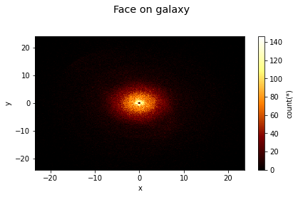
The simplest case is a single heatmap created by two axes, specified by the first two arguments:

df.viz.heatmap('x', 'y', title='Face on galaxy', limits='99%')

Multiple plots of the same type

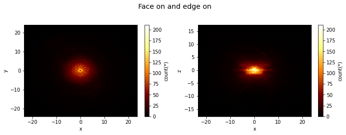
The first argument can be a list of axes pairs. This produces multiple plots:

df.viz.heatmap([["x", "y"], ["x", "z"]], title="Face on and edge on", figsize=(10, 4), limits='99%');

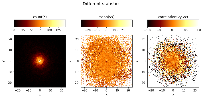
Multiple plots, same axes, different statistics

If the what argument is a list, it will by default create multiple subplots:

df.viz.heatmap("x", "y", what=["count(*)", "mean(vx)", "correlation(vy,vz)"],
               title="Different statistics",
               figsize=(10, 5), limits='99%');

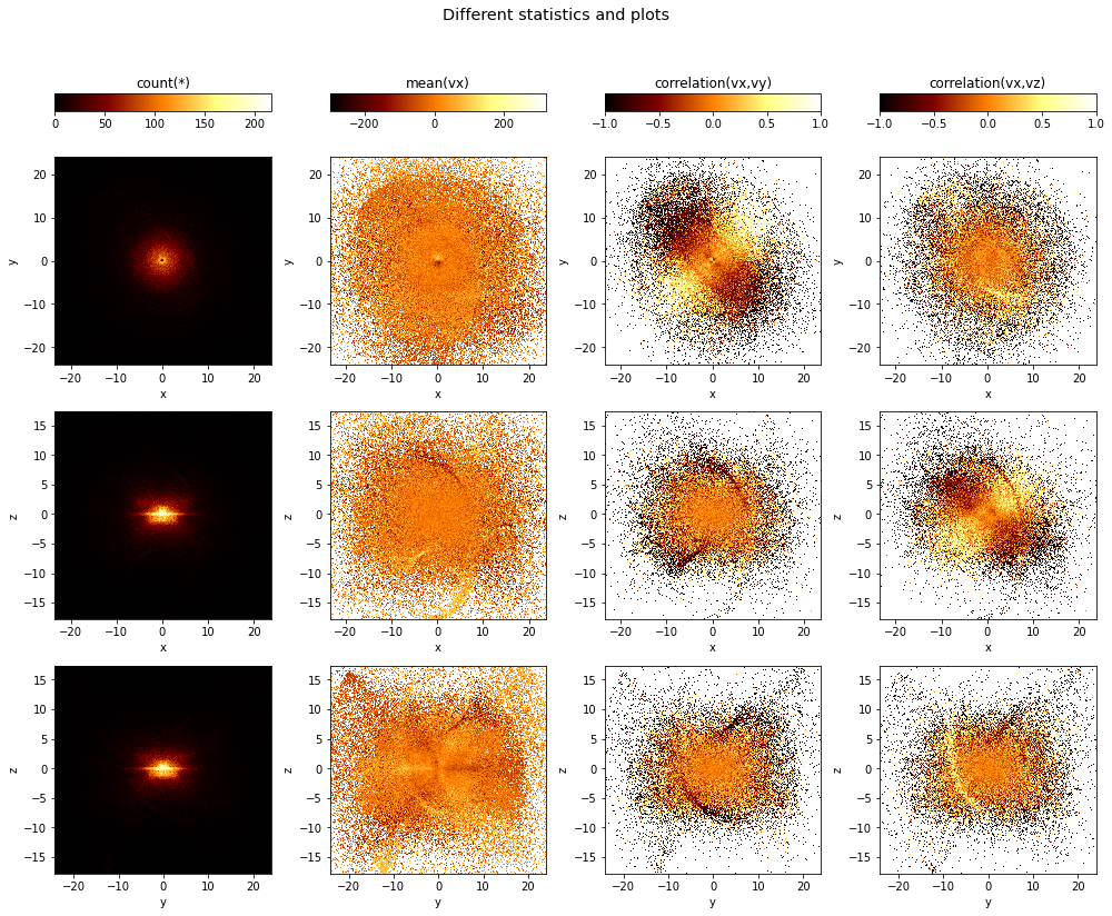
Multiple plots, different axes, different statistics

One can specify multiple axes pairs as tje first argument, as well as a list of what arguments. The resulting figure with have a number of subplots where the different axes combinations will form the rows, and the different what statistics will form the columns:

df.viz.heatmap([["x", "y"], ["x", "z"], ["y", "z"]],
               what=["count(*)", "mean(vx)", "correlation(vx,vy)", "correlation(vx,vz)"],
               title="Different statistics and plots",
               figsize=(14,12),
               limits='99%');

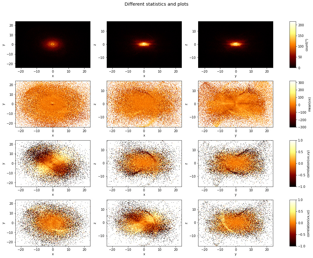
One can also specify the layout of the figure via the visual argument, which can be used to swap the row and column ordering of the subplots:

df.viz.heatmap([["x", "y"], ["x", "z"], ["y", "z"]],
               what=["count(*)", "mean(vx)", "correlation(vx,vy)", "correlation(vx,vz)"],
               visual=dict(row="what", column="subspace"),
               title="Different statistics and plots",
               figsize=(14,12),
               limits='99%');

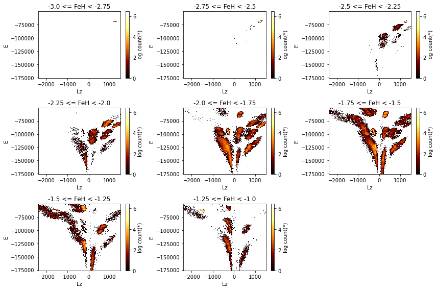
Slices in a 3rd dimension

If a 3rd axis (z) is given, you can “slice” through the data, displaying the z slices as rows. Note that here the rows are wrapped, which can be changed with the wrap_columns argument:

df.viz.heatmap("Lz", "E", z="FeH:-3,-1,8",
               visual=dict(row="z"),
               figsize=(12, 8),
               f="log",
               wrap_columns=3,
               limits='99%');

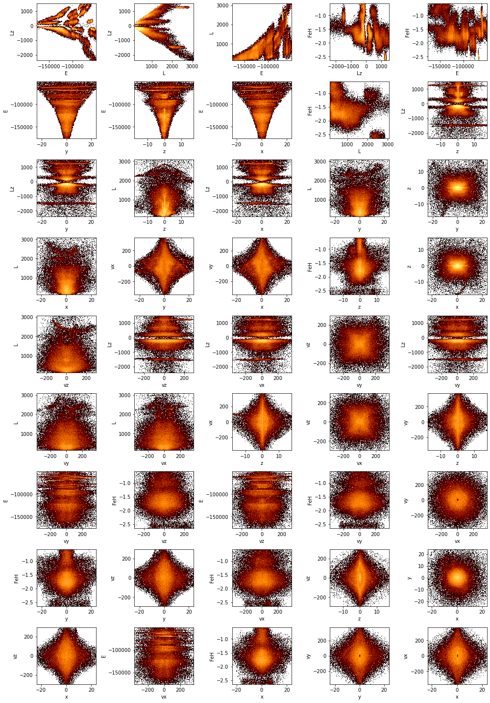
Many plots with wrapping

If one attempt to create a figure with many subplots, they will be nice wrapped. Where we create heatmaps of all combinations of columns in the example dataset, sorted by their mutual information:

# Get all column pars
pairs = df.combinations(exclude=['id'])
# Calculate the mutual information for each pair, sorted by the largest value
mi, pairs_sorted = df.mutual_information(pairs, sort=True)

# Create the figure
df.viz.heatmap(pairs_sorted, f='log', colorbar=False, figsize=(14, 20), limits='99%', wrap_columns=5);

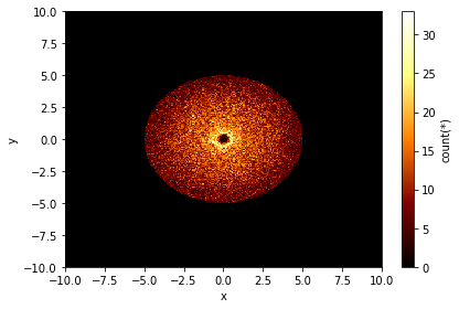
Plotting selections

If the selection argument is used, than only the selection is plotted:

df.viz.heatmap("x", "y", selection="sqrt(x**2+y**2) < 5", limits=[-10, 10]);

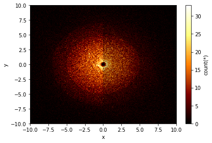
If a list of selections is specified (False or None indicates no selection), than every selection by default forms a different “layer” of the figure produced:

df.viz.heatmap("x", "y",
               selection=[None, "sqrt(x**2+y**2) < 5", "(sqrt(x**2+y**2) < 7) & (x < 0)"],
               limits=[-10, 10]);

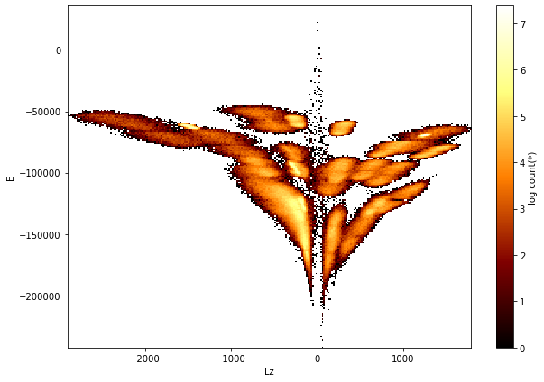
Overplotting a vector field on a heatmap

Astronomers argue that galaxies such as our own Milky Way were formed from many pre-galactic clumps that have merged and mixed together. One way to try and find the original pre-galactic fragments is to inspect the 2-dimensinoal distribution of their energy (𝐸) and angular momentum (𝐿𝑧). So let us make such a plot:

df.viz.heatmap('Lz', 'E', f='log', figsize=(9, 6));

Now, to show that the stars in each clump on the figure above are indeed moving coherently in space, we can overplot their velocity vectors on a positional heatmap.

First, let’s select the stars that belong to one the clusters:

# specify ranges of angular momentum (Lz) and energy (E)
limits_Lz_E_clump = (1181.770, 1291.92), (-70850.91, -68491.16)

# Use the rectangle selection method
df.select_rectangle("Lz", "E", limits_Lz_E_clump, name="stream")

# Check how many stars we have selected
print(f'Selection contains {df.count(selection="stream")} "stars".')

Selection contains 9556 "stars".

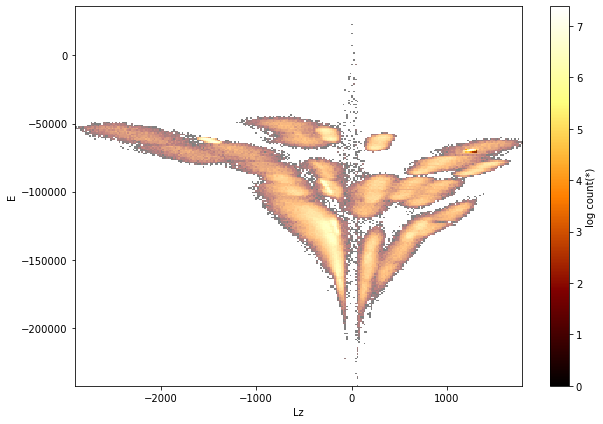
We can also overplot the selected region, to convince ourselves that we have chosen a good region:

df.viz.heatmap("Lz", "E", selection=[None, "stream"], f="log", figsize=(9, 6));

Now let us plot the 𝑣𝑦 and 𝑣𝑧 velocity vectors on top of 𝑦−𝑧 plot. To start, lets compute a grid of mean 𝑣𝑦 and 𝑣𝑧 velocities. Notice that we are limiting the range of the 𝑣𝑦 and 𝑣𝑧 values to go between -20 and 20, and the grid resolution is 32x32 bins:

limits = [-20, 20]
shape_vector = 32
mean_vy = df.mean("vy", binby=["y", "z"], limits=limits, shape=shape_vector, selection='stream')
mean_vz = df.mean("vz", binby=["y", "z"], limits=limits, shape=shape_vector, selection='stream')

Next, let us create a meshgrid to hold the centres of the bins:

# create a 2d array with holds the center of the bins
centers = np.linspace(*limits, shape_vector, endpoint=False) + (limits[1] - limits[0])/2./shape_vector
z, y = np.meshgrid(centers, centers)

To keep the plot “clean”, we also do not want visualize the velocity of the bins with low number counts:

# we don't want to show bins with low number of counts
counts = df.count(binby=["y", "z"], limits=limits, shape=shape_vector, selection='stream')
mask = counts.flatten( ) > 10

Finally we can plot a background density map of \(v_y\) vs \(v_z\), and then use plt.quiver to overplot the velocity vectors:

df.viz.heatmap("y", "z", limits=limits, f="log1p", figsize=(10, 9), selection=[None, "stream"], shape=128)

# overplot the mean velocity vectors
plt.quiver(y.flatten()[mask],
           z.flatten()[mask],
           mean_vy.flatten()[mask],
           mean_vz.flatten()[mask],
           color="white",
           alpha=0.75);

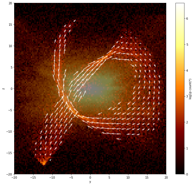
We indeed see that the stars we selected move together, and form a stream!

Plotting a healpix map

Healpix is made available via the healpy package. Vaex does not need special support for healpix, but some helper functions are introduced to make working with healpix easier.

Make sure you have healpy installed. If you do not, you can install it with one of these commands:

!pip install healpy  # if you prefer pip
!conda install -c conda-forge healpy if you are using a conda package manager

To understand this better, we will start from the beginning. If we want to make a density sky plot, we would like to pass to healpy a 1d numpy array where each value represents the density at a location of the sphere, where the location is determined by the array size (the healpix level) and the offset (the location).

This example uses a simulated Gaia dataset. The Gaia data includes the healpix index encoded in the source_id column. By diving source_id by 34359738368 you get a healpix index level 12, and diving it further will take you to lower levels.

Let us start by fetching the dataset (Note: the dataset is ~700MB on disk).

import healpy as hp

df = vaex.datasets.tgas(full=True)
df.head()

#	astrometric_delta_q	astrometric_excess_noise	astrometric_excess_noise_sig	astrometric_n_bad_obs_ac	astrometric_n_bad_obs_al	astrometric_n_good_obs_ac	astrometric_n_good_obs_al	astrometric_n_obs_ac	astrometric_n_obs_al	astrometric_primary_flag	astrometric_priors_used	astrometric_relegation_factor	astrometric_weight_ac	astrometric_weight_al	b	dec	dec_error	dec_parallax_corr	dec_pmdec_corr	dec_pmra_corr	duplicated_source	ecl_lat	ecl_lon	hip	l	matched_observations	parallax	parallax_error	parallax_pmdec_corr	parallax_pmra_corr	phot_g_mean_flux	phot_g_mean_flux_error	phot_g_mean_mag	phot_g_n_obs	phot_variable_flag	pmdec	pmdec_error	pmra	pmra_error	pmra_pmdec_corr	ra	ra_dec_corr	ra_error	ra_parallax_corr	ra_pmdec_corr	ra_pmra_corr	random_index	ref_epoch	scan_direction_mean_k1	scan_direction_mean_k2	scan_direction_mean_k3	scan_direction_mean_k4	scan_direction_strength_k1	scan_direction_strength_k2	scan_direction_strength_k3	scan_direction_strength_k4	solution_id	source_id	tycho2_id
0	1.91906	0.717101	412.606	1	0	78	79	79	79	84	3	2.9361	1.26696e-05	1.81816	-48.7144	0.235392	0.218802	-0.407338	0.0606588	-0.0994513	70	-16.1211	42.6418	13989	176.74	9	6.35295	0.30791	-0.101957	-0.00157679	1.03123e+07	10577.4	7.99138	77	b'NOT_AVAILABLE'	-7.64199	0.0874018	43.7523	0.0705422	0.214677	45.0343	-0.414972	0.305989	0.179966	-0.0857597	0.159207	243619	2015	-113.76	21.3929	-41.6784	26.2018	0.382348	0.538266	0.392379	0.916306	1635378410781933568	7627862074752	b''
1	nan	0.253463	47.3163	2	0	55	57	57	57	84	5	2.65231	3.16002e-05	12.8616	-48.645	0.200068	1.19779	0.837626	-0.975644	0.972577	70	-16.193	42.7612	-2147483648	176.916	8	3.90033	0.323488	-0.853779	0.839739	949565	1140.17	10.581	62	b'NOT_AVAILABLE'	-55.1092	2.52293	10.0363	4.61141	-0.996399	45.165	-0.995923	2.58388	-0.860911	0.97348	-0.972417	487238	2015	-156.433	22.7661	-36.2397	22.8906	0.711003	0.96597	0.646115	0.86716	1635378410781933568	9277129363072	b'55-28-1'
2	nan	0.398901	221.185	4	1	57	60	61	61	84	5	3.9934	2.56339e-05	5.76753	-48.6678	0.248825	0.180326	-0.391891	-0.193256	0.0894205	70	-16.1234	42.6975	-2147483648	176.78	7	3.15531	0.273484	-0.118552	-0.0418587	817838	1827.38	10.7431	60	b'NOT_AVAILABLE'	-1.60287	1.03526	2.93228	1.90864	-0.914271	45.0862	-0.177443	0.213836	0.307722	-0.184817	0.0468668	1948952	2015	-117.008	19.7722	-43.1082	26.7157	0.482528	0.428758	0.524153	0.903062	1635378410781933568	13297218905216	b'55-1191-1'
3	nan	0.422492	179.982	1	0	51	52	52	52	84	5	4.21516	2.86726e-05	5.36086	-48.6824	0.248211	0.200958	-0.337217	-0.223501	0.131811	70	-16.1182	42.6778	-2147483648	176.76	7	2.29237	0.280972	-0.109202	-0.0494409	602053	905.877	11.0757	61	b'NOT_AVAILABLE'	-18.4149	1.12985	3.66198	2.06505	-0.926177	45.0665	-0.365707	0.276039	0.202878	-0.0589288	-0.0509089	102321	2015	-132.421	22.5693	-38.9545	25.8786	0.494655	0.638456	0.509074	0.898918	1635378410781933568	13469017597184	b'55-624-1'
4	nan	0.3175	119.748	2	3	85	84	87	87	84	5	3.23564	2.22788e-05	8.08078	-48.572	0.335044	0.17013	-0.438708	-0.279349	0.121792	70	-16.0555	42.7734	-2147483648	176.739	11	1.58208	0.261539	-0.329196	0.100312	1.38812e+06	2826.43	10.1687	96	b'NOT_AVAILABLE'	-2.37939	0.710632	0.340802	1.22048	-0.833604	45.136	-0.0490526	0.170697	0.471425	-0.156392	-0.152076	409284	2015	-106.86	4.4521	-47.8954	26.7555	0.520654	0.23931	0.653377	0.863385	1635378410781933568	15736760328576	b'55-849-1'
5	nan	0.303723	64.6868	2	1	68	69	70	70	84	5	3.10892	2.22511e-05	9.65279	-48.5511	0.359618	0.179848	-0.437142	-0.376402	0.257906	70	-16.0335	42.7861	-2147483648	176.718	9	8.66308	0.255867	-0.297309	0.0791063	1.66384e+06	1381.58	9.97199	76	b'NOT_AVAILABLE'	-72.7114	0.720852	-52.8493	1.26429	-0.852784	45.1414	-0.264588	0.205008	0.39493	0.102073	-0.36853	204642	2015	-127.824	16.3828	-44.2417	25.1631	0.522809	0.479366	0.621515	0.847412	1635378410781933568	16527034310784	b'55-182-1'
6	nan	0.340405	118.911	2	1	76	77	78	78	84	5	3.44745	2.19728e-05	7.91894	-48.5242	0.386343	0.17188	-0.341053	-0.34408	0.1516	70	-16.0114	42.8058	-2147483648	176.701	9	5.6982	0.263677	-0.367848	0.0846782	1.821e+06	2755.91	9.874	77	b'NOT_AVAILABLE'	-3.35036	0.707184	24.5272	1.17738	-0.800098	45.153	-0.0412512	0.189524	0.488929	-0.163855	-0.195289	540954	2015	-114.478	11.0431	-46.4507	26.2651	0.512088	0.322961	0.637399	0.856398	1635378410781933568	16733192740608	b'55-867-1'
7	nan	0.253709	88.6261	3	0	76	79	79	79	84	5	2.65453	2.57372e-05	13.709	-48.5569	0.380844	0.150943	-0.139315	-0.358996	0.238914	70	-16.0049	42.7641	-2147483648	176.665	10	2.09081	0.222206	-0.277202	0.093748	967144	601.802	10.561	87	b'NOT_AVAILABLE'	-11.6616	0.982994	-1.57293	1.73319	-0.904223	45.1128	-0.187136	0.206981	0.412381	0.0994892	-0.284353	1081909	2015	-88.3027	14.7861	-47.9744	27.0228	0.39079	0.333692	0.400387	0.90071	1635378410781933568	16870631694208	b'55-72-1'
8	nan	0.401473	226.044	3	1	69	71	72	72	84	5	4.01755	2.45771e-05	5.41389	-48.6511	0.351099	0.169345	-0.276625	-0.175754	0.101633	70	-16.0034	42.6531	-2147483648	176.589	9	6.20249	0.247253	-0.139338	0.0669677	1.66582e+06	1233.43	9.9707	79	b'NOT_AVAILABLE'	9.19541	1.02832	26.308	2.03485	-0.905496	45.0103	-0.321544	0.243576	0.263603	-0.143727	0.107397	589318	2015	-106.23	19.3449	-44.7095	25.5226	0.335982	0.520842	0.35827	0.90504	1635378410781933568	26834955821312	b'55-912-1'
9	nan	0.235866	49.3216	2	0	51	53	53	53	84	5	2.49518	2.42543e-05	15.7304	-48.5912	0.473472	0.163531	-0.0605532	-0.242013	0.14566	70	-15.8759	42.6549	-2147483648	176.419	8	1.67767	0.222067	-0.18584	0.0668122	1.96682e+06	1184.17	9.79036	62	b'NOT_AVAILABLE'	-24.5264	1.1319	9.10421	2.20939	-0.92529	44.9747	-0.407078	0.267911	0.236157	-0.0912424	0.0305957	1178636	2015	-99.9696	19.5819	-46.0718	24.0416	0.217998	0.655547	0.219464	0.892649	1635378410781933568	33260226885120	b'48-1139-1'

Let’s plot a healpix figure of level 2. We can start by counting the number of stars in each healpix region:

level = 2
factor = 34359738368 * (4**(12-level))
nmax = hp.nside2npix(2**level)
counts = df.count(binby="source_id/" + str(factor), limits=[0, nmax], shape=nmax)
counts

array([ 4021,  6171,  5318,  7114,  5755, 13420, 12711, 10193,  7782,
       14187, 12578, 22038, 17313, 13064, 17298, 11887,  3859,  3488,
        9036,  5533,  4007,  3899,  4884,  5664, 10741,  7678, 12092,
       10182,  6652,  6793, 10117,  9614,  3727,  5849,  4028,  5505,
        8462, 10059,  6581,  8282,  4757,  5116,  4578,  5452,  6023,
        8340,  6440,  8623,  7308,  6197, 21271, 23176, 12975, 17138,
       26783, 30575, 31931, 29697, 17986, 16987, 19802, 15632, 14273,
       10594,  4807,  4551,  4028,  4357,  4067,  4206,  3505,  4137,
        3311,  3582,  3586,  4218,  4529,  4360,  6767,  7579, 14462,
       24291, 10638, 11250, 29619,  9678, 23322, 18205,  7625,  9891,
        5423,  5808, 14438, 17251,  7833, 15226,  7123,  3708,  6135,
        4110,  3587,  3222,  3074,  3941,  3846,  3402,  3564,  3425,
        4125,  4026,  3689,  4084, 16617, 13577,  6911,  4837, 13553,
       10074,  9534, 20824,  4976,  6707,  5396,  8366, 13494, 19766,
       11012, 16130,  8521,  8245,  6871,  5977,  8789, 10016,  6517,
        8019,  6122,  5465,  5414,  4934,  5788,  6139,  4310,  4144,
       11437, 30731, 13741, 27285, 40227, 16320, 23039, 10812, 14686,
       27690, 15155, 32701, 18780,  5895, 23348,  6081, 17050, 28498,
       35232, 26223, 22341, 15867, 17688,  8580, 24895, 13027, 11223,
        7880,  8386,  6988,  5815,  4717,  9088,  8283, 12059,  9161,
        6952,  4914,  6652,  4666, 12014, 10703, 16518, 10270,  6724,
        4553,  9282,  4981])

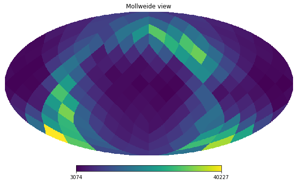
Using the healpy package, we can plot this in a molleweide projection

hp.mollview(counts, nest=True);

To avoid tying the above code all over again, we can use the df.healpix_count method instead:

counts = df.healpix_count(healpix_level=6)
hp.mollview(counts, nest=True)

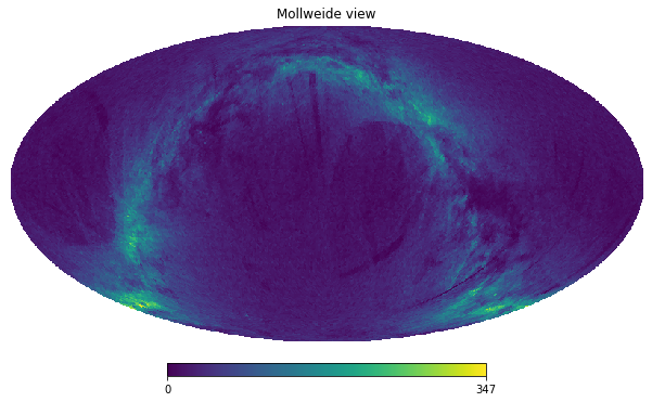
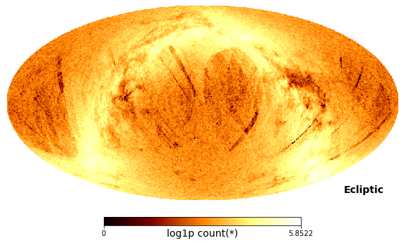
Instead of using healpy, we can use vaex’ df.viz.healpix_plot method:

df.viz.healpix_heatmap(f="log1p", healpix_level=6, figsize=(10,8), healpix_output="ecliptic")

Guides Arrow