![]()
Jupyter integration: interactivity
Vaex can process about 1 billion rows per second, and in combination with the Jupyter notebook, this allows for interactive exporation of large datasets.
Introduction
The vaex-jupyter package contains the building blocks to interactively define an N-dimensional grid, which is then used for visualizations.
We start by defining the building blocks (vaex.jupyter.model.Axis, vaex.jupyter.model.DataArray and vaex.jupyter.view.DataArray) used to define and visualize our N-dimensional grid.
Let us first import the relevant packages, and open the example DataFrame:
[1]:
import vaex
import vaex.jupyter.model as vjm

import numpy as np
import matplotlib.pyplot as plt

df = vaex.example()
df
[1]:
| # | id | x | y | z | vx | vy | vz | E | L | Lz | FeH |
|---|---|---|---|---|---|---|---|---|---|---|---|
| 0 | 0 | 1.2318683862686157 | -0.39692866802215576 | -0.598057746887207 | 301.1552734375 | 174.05947875976562 | 27.42754554748535 | -149431.40625 | 407.38897705078125 | 333.9555358886719 | -1.0053852796554565 |
| 1 | 23 | -0.16370061039924622 | 3.654221296310425 | -0.25490644574165344 | -195.00022888183594 | 170.47216796875 | 142.5302276611328 | -124247.953125 | 890.2411499023438 | 684.6676025390625 | -1.7086670398712158 |
| 2 | 32 | -2.120255947113037 | 3.326052665710449 | 1.7078403234481812 | -48.63423156738281 | 171.6472930908203 | -2.079437255859375 | -138500.546875 | 372.2410888671875 | -202.17617797851562 | -1.8336141109466553 |
| 3 | 8 | 4.7155890464782715 | 4.5852508544921875 | 2.2515437602996826 | -232.42083740234375 | -294.850830078125 | 62.85865020751953 | -60037.0390625 | 1297.63037109375 | -324.6875 | -1.4786882400512695 |
| 4 | 16 | 7.21718692779541 | 11.99471664428711 | -1.064562201499939 | -1.6891745328903198 | 181.329345703125 | -11.333610534667969 | -83206.84375 | 1332.7989501953125 | 1328.948974609375 | -1.8570483922958374 |
| ... | ... | ... | ... | ... | ... | ... | ... | ... | ... | ... | ... |
| 329,995 | 21 | 1.9938701391220093 | 0.789276123046875 | 0.22205990552902222 | -216.92990112304688 | 16.124420166015625 | -211.244384765625 | -146457.4375 | 457.72247314453125 | 203.36758422851562 | -1.7451677322387695 |
| 329,996 | 25 | 3.7180912494659424 | 0.721337616443634 | 1.6415337324142456 | -185.92160034179688 | -117.25082397460938 | -105.4986572265625 | -126627.109375 | 335.0025634765625 | -301.8370056152344 | -0.9822322130203247 |
| 329,997 | 14 | 0.3688507676124573 | 13.029608726501465 | -3.633934736251831 | -53.677146911621094 | -145.15771484375 | 76.70909881591797 | -84912.2578125 | 817.1375732421875 | 645.8507080078125 | -1.7645612955093384 |
| 329,998 | 18 | -0.11259264498949051 | 1.4529125690460205 | 2.168952703475952 | 179.30865478515625 | 205.79710388183594 | -68.75872802734375 | -133498.46875 | 724.000244140625 | -283.6910400390625 | -1.8808952569961548 |
| 329,999 | 4 | 20.796220779418945 | -3.331387758255005 | 12.18841552734375 | 42.69000244140625 | 69.20479583740234 | 29.54275131225586 | -65519.328125 | 1843.07470703125 | 1581.4151611328125 | -1.1231083869934082 |
We want to build a 2 dimensinoal grid with the number counts in each bin. To do this, we first define two axis objects:
[2]:
E_axis = vjm.Axis(df=df, expression=df.E, shape=140)
Lz_axis = vjm.Axis(df=df, expression=df.Lz, shape=100)
Lz_axis
[2]:
Axis(bin_centers=None, exception=None, expression=Lz, max=None, min=None, shape=100, shape_default=64, slice=None, status=Status.NO_LIMITS)
When we inspect the Lz_axis object we see that the min, max, and bin centers are all None. This is because Vaex calculates them in the background, so the kernel stays interactive, meaning you can continue working in the notebook. We can ask Vaex to wait until all background calculations are done. Note that for billions of rows, this can take over a second.
[3]:
await vaex.jupyter.gather()  # wait until Vaex is done with all background computation
Lz_axis  # now min and max are computed, and bin_centers is set
[3]:
Axis(bin_centers=[-2877.11808899 -2830.27174744 -2783.42540588 -2736.57906433
 -2689.73272278 -2642.88638123 -2596.04003967 -2549.19369812
 -2502.34735657 -2455.50101501 -2408.65467346 -2361.80833191
 -2314.96199036 -2268.1156488  -2221.26930725 -2174.4229657
 -2127.57662415 -2080.73028259 -2033.88394104 -1987.03759949
 -1940.19125793 -1893.34491638 -1846.49857483 -1799.65223328
 -1752.80589172 -1705.95955017 -1659.11320862 -1612.26686707
 -1565.42052551 -1518.57418396 -1471.72784241 -1424.88150085
 -1378.0351593  -1331.18881775 -1284.3424762  -1237.49613464
 -1190.64979309 -1143.80345154 -1096.95710999 -1050.11076843
 -1003.26442688  -956.41808533  -909.57174377  -862.72540222
  -815.87906067  -769.03271912  -722.18637756  -675.34003601
  -628.49369446  -581.64735291  -534.80101135  -487.9546698
  -441.10832825  -394.26198669  -347.41564514  -300.56930359
  -253.72296204  -206.87662048  -160.03027893  -113.18393738
   -66.33759583   -19.49125427    27.35508728    74.20142883
   121.04777039   167.89411194   214.74045349   261.58679504
   308.4331366    355.27947815   402.1258197    448.97216125
   495.81850281   542.66484436   589.51118591   636.35752747
   683.20386902   730.05021057   776.89655212   823.74289368
   870.58923523   917.43557678   964.28191833  1011.12825989
  1057.97460144  1104.82094299  1151.66728455  1198.5136261
  1245.35996765  1292.2063092   1339.05265076  1385.89899231
  1432.74533386  1479.59167542  1526.43801697  1573.28435852
  1620.13070007  1666.97704163  1713.82338318  1760.66972473], exception=None, expression=Lz, max=1784.0928955078125, min=-2900.541259765625, shape=100, shape_default=64, slice=None, status=Status.READY)
Note that the Axis is a traitlets HasTrait object, similar to all ipywidget objects. This means that we can link all of its properties to an ipywidget and thus creating interactivity. We can also use observe to listen to any changes to our model.
An interactive xarray DataArray display
Now that we have defined our two axes, we can create a vaex.jupyter.model.DataArray (model) together with a vaex.jupyter.view.DataArray (view).
A convenient way to do this, is to use the widget accessor data_array method, which creates both, links them together and will return a view for us.
The returned view is an ipywidget object, which becomes a visual element in the Jupyter notebook when displayed.
[4]:
data_array_widget = df.widget.data_array(axes=[Lz_axis, E_axis], selection=[None, 'default'])
data_array_widget  # being the last expression in the cell, Jupyter  will 'display' the widget
Note: If you see this notebook on readthedocs, you will see the selection coordinate already has ``[None, ‘default’]``, because cells below have already been executed and have updated this widget. If you run this notebook yourself (say on mybinder), you will see after executing the above cell, the selection will have ``[None]`` as its only value.
From the specification of the axes and the selections, Vaex computes a 3d histogram, the first dimension being the selections. Interally this is simply a numpy array, but we wrap it in an xarray DataArray object. An xarray DataArray object can be seen as a labeled Nd array, i.e. a numpy array with extra metadata to make it fully self-describing.
Notice that in the above code cell, we specified the selection argument with a list containing two elements in this case, None and 'default'. The None selection simply shows all the data, while the default refers to any selection made without explicitly naming it. Even though the later has not been defined at this point, we can still pre-emptively include it, in case we want to modify it later.
The most important properties of the data_array are printed out below:
[5]:
# NOTE: since the computations are done in the background, data_array_widget.model.grid is initially None.
# We can ask vaex-jupyter to wait till all executions are done using:
await vaex.jupyter.gather()
# get a reference to the xarray DataArray object
data_array = data_array_widget.model.grid
print(f"type:", type(data_array))
print("dims:", data_array.dims)
print("data:", data_array.data)
print("coords:", data_array.coords)
print("Lz's data:", data_array.coords['Lz'].data)
print("Lz's attrs:", data_array.coords['Lz'].attrs)
print("And displaying the xarray DataArray:")
display(data_array)  # this is what the vaex.jupyter.view.DataArray uses
type: <class 'xarray.core.dataarray.DataArray'>
dims: ('selection', 'Lz', 'E')
data: [[[0 0 0 ... 0 0 0]
  [0 0 0 ... 0 0 0]
  [0 0 0 ... 0 0 0]
  ...
  [0 0 0 ... 0 0 0]
  [0 0 0 ... 0 0 0]
  [0 0 0 ... 0 0 0]]]
coords: Coordinates:
  * selection  (selection) object None
  * Lz         (Lz) float64 -2.877e+03 -2.83e+03 ... 1.714e+03 1.761e+03
  * E          (E) float64 -2.414e+05 -2.394e+05 ... 3.296e+04 3.495e+04
Lz's data: [-2877.11808899 -2830.27174744 -2783.42540588 -2736.57906433
 -2689.73272278 -2642.88638123 -2596.04003967 -2549.19369812
 -2502.34735657 -2455.50101501 -2408.65467346 -2361.80833191
 -2314.96199036 -2268.1156488  -2221.26930725 -2174.4229657
 -2127.57662415 -2080.73028259 -2033.88394104 -1987.03759949
 -1940.19125793 -1893.34491638 -1846.49857483 -1799.65223328
 -1752.80589172 -1705.95955017 -1659.11320862 -1612.26686707
 -1565.42052551 -1518.57418396 -1471.72784241 -1424.88150085
 -1378.0351593  -1331.18881775 -1284.3424762  -1237.49613464
 -1190.64979309 -1143.80345154 -1096.95710999 -1050.11076843
 -1003.26442688  -956.41808533  -909.57174377  -862.72540222
  -815.87906067  -769.03271912  -722.18637756  -675.34003601
  -628.49369446  -581.64735291  -534.80101135  -487.9546698
  -441.10832825  -394.26198669  -347.41564514  -300.56930359
  -253.72296204  -206.87662048  -160.03027893  -113.18393738
   -66.33759583   -19.49125427    27.35508728    74.20142883
   121.04777039   167.89411194   214.74045349   261.58679504
   308.4331366    355.27947815   402.1258197    448.97216125
   495.81850281   542.66484436   589.51118591   636.35752747
   683.20386902   730.05021057   776.89655212   823.74289368
   870.58923523   917.43557678   964.28191833  1011.12825989
  1057.97460144  1104.82094299  1151.66728455  1198.5136261
  1245.35996765  1292.2063092   1339.05265076  1385.89899231
  1432.74533386  1479.59167542  1526.43801697  1573.28435852
  1620.13070007  1666.97704163  1713.82338318  1760.66972473]
Lz's attrs: {'min': -2900.541259765625, 'max': 1784.0928955078125}
And displaying the xarray DataArray:
- selection: 1
- Lz: 100
- E: 140
- 0 0 0 0 0 0 0 0 0 0 0 0 0 0 0 0 0 ... 0 0 0 0 0 0 0 0 0 0 0 0 0 0 0 0
array([[[0, 0, 0, ..., 0, 0, 0], [0, 0, 0, ..., 0, 0, 0], [0, 0, 0, ..., 0, 0, 0], ..., [0, 0, 0, ..., 0, 0, 0], [0, 0, 0, ..., 0, 0, 0], [0, 0, 0, ..., 0, 0, 0]]]) - selection(selection)objectNone
array([None], dtype=object)
- Lz(Lz)float64-2.877e+03 -2.83e+03 ... 1.761e+03
- min :
- -2900.541259765625
- max :
- 1784.0928955078125
array([-2877.118089, -2830.271747, -2783.425406, -2736.579064, -2689.732723, -2642.886381, -2596.04004 , -2549.193698, -2502.347357, -2455.501015, -2408.654673, -2361.808332, -2314.96199 , -2268.115649, -2221.269307, -2174.422966, -2127.576624, -2080.730283, -2033.883941, -1987.037599, -1940.191258, -1893.344916, -1846.498575, -1799.652233, -1752.805892, -1705.95955 , -1659.113209, -1612.266867, -1565.420526, -1518.574184, -1471.727842, -1424.881501, -1378.035159, -1331.188818, -1284.342476, -1237.496135, -1190.649793, -1143.803452, -1096.95711 , -1050.110768, -1003.264427, -956.418085, -909.571744, -862.725402, -815.879061, -769.032719, -722.186378, -675.340036, -628.493694, -581.647353, -534.801011, -487.95467 , -441.108328, -394.261987, -347.415645, -300.569304, -253.722962, -206.87662 , -160.030279, -113.183937, -66.337596, -19.491254, 27.355087, 74.201429, 121.04777 , 167.894112, 214.740453, 261.586795, 308.433137, 355.279478, 402.12582 , 448.972161, 495.818503, 542.664844, 589.511186, 636.357527, 683.203869, 730.050211, 776.896552, 823.742894, 870.589235, 917.435577, 964.281918, 1011.12826 , 1057.974601, 1104.820943, 1151.667285, 1198.513626, 1245.359968, 1292.206309, 1339.052651, 1385.898992, 1432.745334, 1479.591675, 1526.438017, 1573.284359, 1620.1307 , 1666.977042, 1713.823383, 1760.669725]) - E(E)float64-2.414e+05 -2.394e+05 ... 3.495e+04
- min :
- -242407.5
- max :
- 35941.86328125
array([-241413.395131, -239425.185393, -237436.975656, -235448.765918,
       -233460.55618 , -231472.346443, -229484.136705, -227495.926967,
       -225507.717229, -223519.507492, -221531.297754, -219543.088016,
       -217554.878278, -215566.668541, -213578.458803, -211590.249065,
       -209602.039328, -207613.82959 , -205625.619852, -203637.410114,
       -201649.200377, -199660.990639, -197672.780901, -195684.571164,
       -193696.361426, -191708.151688, -189719.94195 , -187731.732213,
       -185743.522475, -183755.312737, -181767.102999, -179778.893262,
       -177790.683524, -175802.473786, -173814.264049, -171826.054311,
       -169837.844573, -167849.634835, -165861.425098, -163873.21536 ,
       -161885.005622, -159896.795884, -157908.586147, -155920.376409,
       -153932.166671, -151943.956934, -149955.747196, -147967.537458,
       -145979.32772 , -143991.117983, -142002.908245, -140014.698507,
       -138026.48877 , -136038.279032, -134050.069294, -132061.859556,
       -130073.649819, -128085.440081, -126097.230343, -124109.020605,
       -122120.810868, -120132.60113 , -118144.391392, -116156.181655,
       -114167.971917, -112179.762179, -110191.552441, -108203.342704,
       -106215.132966, -104226.923228, -102238.713491, -100250.503753,
        -98262.294015,  -96274.084277,  -94285.87454 ,  -92297.664802,
        -90309.455064,  -88321.245326,  -86333.035589,  -84344.825851,
        -82356.616113,  -80368.406376,  -78380.196638,  -76391.9869  ,
        -74403.777162,  -72415.567425,  -70427.357687,  -68439.147949,
        -66450.938211,  -64462.728474,  -62474.518736,  -60486.308998,
        -58498.099261,  -56509.889523,  -54521.679785,  -52533.470047,
        -50545.26031 ,  -48557.050572,  -46568.840834,  -44580.631097,
        -42592.421359,  -40604.211621,  -38616.001883,  -36627.792146,
        -34639.582408,  -32651.37267 ,  -30663.162932,  -28674.953195,
        -26686.743457,  -24698.533719,  -22710.323982,  -20722.114244,
        -18733.904506,  -16745.694768,  -14757.485031,  -12769.275293,
        -10781.065555,   -8792.855818,   -6804.64608 ,   -4816.436342,
         -2828.226604,    -840.016867,    1148.192871,    3136.402609,
          5124.612347,    7112.822084,    9101.031822,   11089.24156 ,
         13077.451297,   15065.661035,   17053.870773,   19042.080511,
         21030.290248,   23018.499986,   25006.709724,   26994.919461,
         28983.129199,   30971.338937,   32959.548675,   34947.758412])
Note that data_array.coords['Lz'].data is the same as Lz_axis.bin_centers and data_array.coords['Lz'].attrs contains the same min/max as the Lz_axis.
Also, we see that displaying the xarray.DataArray object (data_array_view.model.grid) gives us the same output as the data_array_view above. There is a big difference however. If we change a selection:
[6]:
df.select(df.x > 0)
and scroll back we see that the data_array_view widget has updated itself, and now contains two selections! This is a very powerful feature, that allows us to make interactive visualizations.
Interactive plots
To make interactive plots we can pass a custom display_function to the data_array_widget. This will override the default notebook behaviour which is a call to display(data_array_widget). In the following example we create a function that displays a matplotlib figure:
[7]:
# NOTE: da is short for 'data array'
def plot2d(da):
    plt.figure(figsize=(8, 8))
    ar = da.data[1]  # take the numpy data, and select take the selection
    print(f'imshow of a numpy array of shape: {ar.shape}')
    plt.imshow(np.log1p(ar.T), origin='lower')

df.widget.data_array(axes=[Lz_axis, E_axis], display_function=plot2d, selection=[None, True])
In the above figure, we choose index 1 along the selection axis, which referes to the 'default' selection. Choosing an index of 0 would correspond to the None selection, and all the data would be displayed. If we now change the selection, the figure will update itself:
[8]:
df.select(df.id < 10)
As xarray’s DataArray is fully self describing, we can improve the plot by using the dimension names for labeling, and setting the extent of the figure’s axes.
Note that we don’t need any information from the Axis objects created above, and in fact, we should not use them, since they may not be in sync with the xarray DataArray object. Later on, we will create a widget that will edit the Axis’ expression.
Our improved visualization with proper axes and labeling:
[9]:
def plot2d_with_labels(da):
    plt.figure(figsize=(8, 8))
    grid = da.data  # take the numpy data
    dim_x = da.dims[0]
    dim_y = da.dims[1]
    plt.title(f'{dim_y} vs {dim_x} - shape: {grid.shape}')
    extent = [
        da.coords[dim_x].attrs['min'], da.coords[dim_x].attrs['max'],
        da.coords[dim_y].attrs['min'], da.coords[dim_y].attrs['max']
    ]
    plt.imshow(np.log1p(grid.T), origin='lower', extent=extent, aspect='auto')
    plt.xlabel(da.dims[0])
    plt.ylabel(da.dims[1])

da_plot_view_nicer = df.widget.data_array(axes=[Lz_axis, E_axis], display_function=plot2d_with_labels)
da_plot_view_nicer
We can also create more sophisticated plots, for example one where we show all of the selections. Note that we can pre-emptively expect a selection and define it later:
[10]:
def plot2d_with_selections(da):
    grid = da.data
    # Create 1 row and #selections of columns of matplotlib axes
    fig, axgrid = plt.subplots(1, grid.shape[0], sharey=True, squeeze=False)
    for selection_index, ax in enumerate(axgrid[0]):
        ax.imshow(np.log1p(grid[selection_index].T), origin='lower')

df.widget.data_array(axes=[Lz_axis, E_axis], display_function=plot2d_with_selections,
                     selection=[None, 'default', 'rest'])
Modifying a selection will update the figure.
[11]:
df.select(df.id < 10)  # select 10 objects
df.select(df.id >= 10, name='rest')  # and the rest
Another advantage of using xarray is its excellent plotting capabilities. It handles a lot of the boring stuff like axis labeling, and also provides a nice interface for slicing the data even more.
Let us introduce another axis, FeH (fun fact: FeH is a property of stars that tells us how much iron relative to hydrogen is contained in them, an idicator of their origin):
[12]:
FeH_axis = vjm.Axis(df=df, expression='FeH', min=-3, max=1, shape=5)
da_view = df.widget.data_array(axes=[E_axis, Lz_axis, FeH_axis], selection=[None, 'default'])
da_view
We can see that we now have a 4 dimensional grid, which we would like to visualize.
And xarray’s plot make our life much easier:
[13]:
def plot_with_xarray(da):
    da_log = np.log1p(da)  # Note that an xarray DataArray is like a numpy array
    da_log.plot(x='Lz', y='E', col='FeH', row='selection', cmap='viridis')

plot_view = df.widget.data_array([E_axis, Lz_axis, FeH_axis], display_function=plot_with_xarray,
                                 selection=[None, 'default', 'rest'])
plot_view
We only have to tell xarray which axis it should map to which ‘aesthetic’, speaking in Grammar of Graphics terms.
Selection widgets
Although we can change the selection in the notebook (e.g. df.select(df.id > 20)), if we create a dashboard (using Voila) we cannot execute arbitrary code. Vaex-jupyter also comes with many widgets, and one of them is a selection_expression widget:
[14]:
selection_widget = df.widget.selection_expression()
selection_widget
The counter_selection creates a widget which keeps track of the number of rows in a selection. In this case we ask it to be ‘lazy’, which means that it will not cause extra passes over the data, but will ride along if some user action triggers a calculation.
[15]:
await vaex.jupyter.gather()
w = df.widget.counter_selection('default', lazy=True)
w
Axis control widgets
Let us create new axis objects using the same expressions as before, but give them more general names (x_axis and y_axis), because we want to change the expressions interactively.
[16]:
x_axis = vjm.Axis(df=df, expression=df.Lz)
y_axis = vjm.Axis(df=df, expression=df.E)

da_xy_view = df.widget.data_array(axes=[x_axis, y_axis], display_function=plot2d_with_labels, shape=180)
da_xy_view
Again, we can change the expressions of the axes programmatically:
[17]:
# wait for the previous plot to finish
await vaex.jupyter.gather()
# Change both the x and y axis
x_axis.expression = np.log(df.x**2)
y_axis.expression = df.y
# Note that both assignment will create 1 computation in the background (minimal amount of passes over the data)
await vaex.jupyter.gather()
# vaex computed the new min/max, and the xarray DataArray
# x_axis.min, x_axis.max, da_xy_view.model.grid
But, if we want to create a dashboard with Voila, we need to have a widget that controls them:
[18]:
x_widget = df.widget.expression(x_axis.expression, label='X axis')
x_widget
This widget will allow us to edit an expression, which will be validated by Vaex. How do we ‘link’ the value of the widget to the axis expression? Because both the Axis as well as the x_widget are HasTrait objects, we can link their traits together:
[19]:
from ipywidgets import link
link((x_widget, 'value'), (x_axis, 'expression'))
[19]:
<traitlets.traitlets.link at 0x122bed450>
Since this operation is so common, we can also directly pass the Axis object, and Vaex will set up the linking for us:
[20]:
y_widget = df.widget.expression(y_axis, label='X axis')
# vaex now does this for us, much shorter
# link((y_widget, 'value'), (y_axis, 'expression'))
y_widget
[21]:
await vaex.jupyter.gather() # lets wait again till all calculations are finished
A nice container
If you are familiar with the ipyvuetify components, you can combine them to create very pretty widgets. Vaex-jupyter comes with a nice container:
[22]:
from vaex.jupyter.widgets import ContainerCard

ContainerCard(title='My plot',
              subtitle="using vaex-jupyter",
              main=da_xy_view,
              controls=[x_widget, y_widget], show_controls=True)
We can directly assign a Vaex expression to the x_axis.expression, or to x_widget.value since they are linked.
[23]:
y_axis.expression = df.vx
Interactive plots
So far we have been using interactive widgets to control the axes in the view. The figure itself however was not interactive, and we could not have panned or zoomed for example.
Vaex has a few builtin visualizations, most notably a heatmap and histogram using bqplot:
[24]:
df = vaex.example()  # we create the dataframe again, to leave all the plots above 'alone'
heatmap_xy = df.widget.heatmap(df.x, df.y, selection=[None, True])
heatmap_xy
Note that we passed expressions, and not axis objects. Vaex recognizes this and will create the axis objects for you. You can access them from the model:
[25]:
heatmap_xy.model.x
[25]:
Axis(bin_centers=[-77.7255446  -76.91058156 -76.09561852 -75.28065547 -74.46569243
 -73.65072939 -72.83576635 -72.0208033  -71.20584026 -70.39087722
 -69.57591417 -68.76095113 -67.94598809 -67.13102505 -66.316062
 -65.50109896 -64.68613592 -63.87117288 -63.05620983 -62.24124679
 -61.42628375 -60.6113207  -59.79635766 -58.98139462 -58.16643158
 -57.35146853 -56.53650549 -55.72154245 -54.90657941 -54.09161636
 -53.27665332 -52.46169028 -51.64672723 -50.83176419 -50.01680115
 -49.20183811 -48.38687506 -47.57191202 -46.75694898 -45.94198593
 -45.12702289 -44.31205985 -43.49709681 -42.68213376 -41.86717072
 -41.05220768 -40.23724464 -39.42228159 -38.60731855 -37.79235551
 -36.97739246 -36.16242942 -35.34746638 -34.53250334 -33.71754029
 -32.90257725 -32.08761421 -31.27265117 -30.45768812 -29.64272508
 -28.82776204 -28.01279899 -27.19783595 -26.38287291 -25.56790987
 -24.75294682 -23.93798378 -23.12302074 -22.3080577  -21.49309465
 -20.67813161 -19.86316857 -19.04820552 -18.23324248 -17.41827944
 -16.6033164  -15.78835335 -14.97339031 -14.15842727 -13.34346423
 -12.52850118 -11.71353814 -10.8985751  -10.08361205  -9.26864901
  -8.45368597  -7.63872293  -6.82375988  -6.00879684  -5.1938338
  -4.37887076  -3.56390771  -2.74894467  -1.93398163  -1.11901858
  -0.30405554   0.5109075    1.32587054   2.14083359   2.95579663
   3.77075967   4.58572271   5.40068576   6.2156488    7.03061184
   7.84557489   8.66053793   9.47550097  10.29046401  11.10542706
  11.9203901   12.73535314  13.55031618  14.36527923  15.18024227
  15.99520531  16.81016836  17.6251314   18.44009444  19.25505748
  20.07002053  20.88498357  21.69994661  22.51490965  23.3298727
  24.14483574  24.95979878  25.77476183  26.58972487  27.40468791
  28.21965095  29.034614    29.84957704  30.66454008  31.47950312
  32.29446617  33.10942921  33.92439225  34.7393553   35.55431834
  36.36928138  37.18424442  37.99920747  38.81417051  39.62913355
  40.4440966   41.25905964  42.07402268  42.88898572  43.70394877
  44.51891181  45.33387485  46.14883789  46.96380094  47.77876398
  48.59372702  49.40869007  50.22365311  51.03861615  51.85357919
  52.66854224  53.48350528  54.29846832  55.11343136  55.92839441
  56.74335745  57.55832049  58.37328354  59.18824658  60.00320962
  60.81817266  61.63313571  62.44809875  63.26306179  64.07802483
  64.89298788  65.70795092  66.52291396  67.33787701  68.15284005
  68.96780309  69.78276613  70.59772918  71.41269222  72.22765526
  73.0426183   73.85758135  74.67254439  75.48750743  76.30247048
  77.11743352  77.93239656  78.7473596   79.56232265  80.37728569
  81.19224873  82.00721177  82.82217482  83.63713786  84.4521009
  85.26706395  86.08202699  86.89699003  87.71195307  88.52691612
  89.34187916  90.1568422   90.97180524  91.78676829  92.60173133
  93.41669437  94.23165742  95.04662046  95.8615835   96.67654654
  97.49150959  98.30647263  99.12143567  99.93639871 100.75136176
 101.5663248  102.38128784 103.19625089 104.01121393 104.82617697
 105.64114001 106.45610306 107.2710661  108.08602914 108.90099218
 109.71595523 110.53091827 111.34588131 112.16084436 112.9758074
 113.79077044 114.60573348 115.42069653 116.23565957 117.05062261
 117.86558565 118.6805487  119.49551174 120.31047478 121.12543783
 121.94040087 122.75536391 123.57032695 124.38529    125.20025304
 126.01521608 126.83017913 127.64514217 128.46010521 129.27506825
 130.0900313 ], exception=None, expression=x, max=130.4975128173828, min=-78.13302612304688, shape=None, shape_default=256, slice=None, status=Status.READY)
The heatmap itself is again a widget. Thus we can combine it with other widgets to create a more sophisticated interface.
[26]:
x_widget = df.widget.expression(heatmap_xy.model.x, label='X axis')
y_widget = df.widget.expression(heatmap_xy.model.y, label='X axis')

ContainerCard(title='My plot',
              subtitle="using vaex-jupyter and bqplot",
              main=heatmap_xy,
              controls=[x_widget, y_widget, selection_widget],
              show_controls=True,
              card_props={'style': 'min-width: 800px;'})
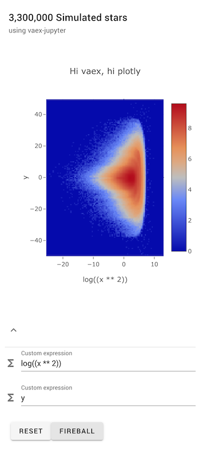
By switching the tool in the toolbar (click pan_tool, or changing it programmmatically in the next cell), we can zoom in. The plot’s axis bounds are directly synched to the axis object (the x_min is linked to the x_axis min, etc). Thus a zoom action causes the axis objects to be changed, which will trigger a recomputation.
[27]:
heatmap_xy.tool = 'pan-zoom' # we can also do this programmatically.
Since we can access the Axis objects, we can also programmatically change the heatmap. Note that both the expression widget, the plot axis label and the heatmap it self is updated. Everything is linked together!
[28]:
heatmap_xy.model.x.expression = np.log10(df.x**2)
await vaex.jupyter.gather()  # and we wait before we continue
Another visualization based on bqplot is the interactive histogram. In the example below, we show all the data, but the selection interaction will affect/set the ‘default’ selection.
[29]:
histogram_Lz = df.widget.histogram(df.Lz, selection_interact='default')
histogram_Lz.tool = 'select-x'
histogram_Lz
[30]:
# You can graphically select a particular region, in this case we do it programmatically
# for reproducability of this notebook
histogram_Lz.plot.figure.interaction.selected = [1200, 1300]
This shows an interesting structure in the heatmap above
Creating your own visualizations
The primary goal of Vaex-Jupyter is to provide users with a framework to create dashboard and new visualizations. Over time more visualizations will go into the vaex-jupyter package, but giving you the option to create new ones is more important. To help you create new visualization, we have examples on how to create your own:
If you want to create your own visualization on this framework, check out these examples:
ipyvolume example